Overview:-
Interpolation and data fitting are two important schemes in data analytics. Interpolation is a type of estimation in which new set of data points are obtained from available range of discrete data sets. It is basically a function approximation which only requires a function and a limited number of independent variables enough to gather the required data or sample for observation. Interpolation can be Piecewise continuous, Linear, Polynomial based or Splined. These are used to understand meaningful patterns in recorded data and deduce future trends.
A Piecewise cubic polyomial interpolation approach is used in this study. The interpolated polynomial using this method is smooth, 2nd order differentiable, has a Not-A-Knot boundary conditions, and converges greatly with reduced error on increasing the number of observation data-points.
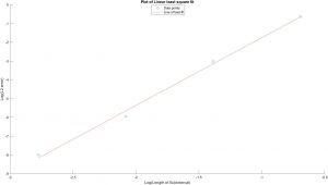
The residual of the L2 norm of the error was plotted against the length of sub-interval on a log-log scale. From the observation of the L2 error plot versus the log of sub-interval, the line of best fit was formed and its slope was determined to be 4th order accurate.
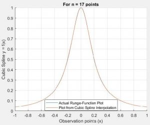
Runge function was used to validate the written MATLAB code of spline interpolation for 5, 9, 17, 33 number of data points.
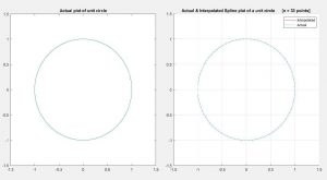
A test case where repeating set of data point on abscissa and ordinates was performed which would generate a circular spline of radius 9 units.
Methodology:-
The spline must have a global smoothness property with Not-A-Knot boundary conditions. Therefore, we must formulate a 3rd order interpolating polynomial such that it has continuous 1st and 2nd derivatives.
- We start with defining the start point, end point and knots in-between. For 'i' number of selected points, we have 'i+1' number of data sets indexed from 0 to 'i+1'.
- Then using the standard formulation for a cubic spline, we apply the conditions of continuity for a cubic 2nd order differentiable spline. This allows us to determine the coefficients of the interpolating polynomial of the spline.
- With having the coefficients determined and plugged back in the polynomial, we can now plot the spline equation for any desired point x(i). This point must lie between two consecutive data knots such that; x(i-1) =< x(i) =< x(i+1) and must not break the continuity of the spline.

Read the project in detail ....